Value at Risk (VaR) Analysis of AAPL Stock

Overview

This project performs a comprehensive Value at Risk (VaR) analysis of Apple Inc. (AAPL) stock, utilizing multiple risk estimation techniques. VaR is a key risk management metric used to estimate the potential loss in value of an asset over a given time period with a specified confidence level. The analysis employs historical VaR, parametric (Gaussian) VaR, and Monte Carlo simulation to assess potential downside risk.

Methodology

1. Data Collection

Retrieves historical stock prices of AAPL from Yahoo Finance using the quantmod package.
Extracts the adjusted closing prices and calculates daily log returns.
Handles missing values and ensures clean financial data.

2. VaR Calculation

Historical VaR: Uses the empirical distribution of past returns to estimate risk.
Parametric VaR: Assumes returns follow a normal distribution and calculates risk based on mean and standard deviation.
Monte Carlo Simulation: Generates 10,000 return simulations based on historical statistics to estimate potential future losses.

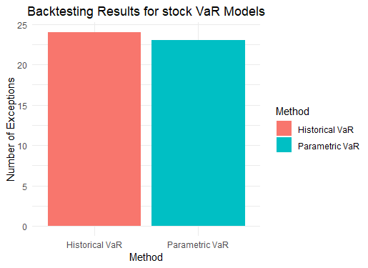
3. Backtesting

Compares actual returns against calculated VaR thresholds.
Counts exceptions where actual losses exceed the estimated VaR, evaluating model accuracy.

4. Visualization

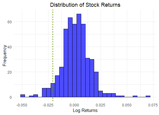
Histogram of Returns: Displays the distribution of AAPL’s daily returns.
VaR Thresholds: Red and green vertical lines indicate the historical and parametric VaR levels, respectively.

Technologies Used

R Programming Language
quantmod – Financial data extraction
PerformanceAnalytics – Risk and return analytics
ggplot2 – Data visualization
dplyr – Data manipulation

Key Insights

The analysis provides an estimation of potential losses for AAPL stock under different market conditions.
Backtesting ensures that the VaR models remain reliable for risk assessment.
Combining multiple VaR methodologies allows for a more robust risk analysis.

Future Improvements

Incorporate conditional VaR (CVaR) for deeper risk assessment.
Extend analysis to multiple assets for portfolio-wide risk management.
Utilize GARCH models to account for volatility clustering in financial time series.

This project demonstrates a quantitative approach to risk management, providing insights into financial market risk using statistical modeling and simulation techniques.

Images:

Value at Risk Forecast

Histogram of Returns + VaR values

Back Testing

Code:

library(quantmod)        # For financial data
library(PerformanceAnalytics) # For VaR calculation
library(ggplot2)         # For visualization
library(dplyr)           # For data manipulation
library(scales)

# Step 1: Data Collection
getSymbols("AAPL", src = "yahoo", from = "2023-01-01", to = Sys.Date())
stock_data <- get("AAPL")

# Calculate daily returns
returns <- dailyReturn(Cl(stock_data), type = "log")  # Log returns
returns <- na.omit(returns)

# Step 2: VaR Calculation
# Historical VaR
historical_VaR <- VaR(returns, p = 0.95, method = "historical")
historical_VaR_value <- as.numeric(historical_VaR)

# Parametric VaR
parametric_VaR <- VaR(returns, p = 0.95, method = "gaussian")
parametric_VaR_value <- as.numeric(parametric_VaR)

# Monte Carlo Simulation (simulating 10,000 returns)
set.seed(123)
simulated_returns <- replicate(10000, {
  mean_return <- mean(returns)
  sd_return <- sd(returns)
  rnorm(length(returns), mean = mean_return, sd = sd_return)
})
monte_carlo_VaR <- apply(simulated_returns, 2, function(x) quantile(x, 0.05))

# Step 3: Backtesting VaR
# Count exceptions for backtesting
exceptions_historical <- sum(returns < historical_VaR_value)
exceptions_parametric <- sum(returns < parametric_VaR_value)

# Step 4: Visualization
# 4.1 Distribution of Returns
ggplot(returns, aes(x = daily.returns)) +
  geom_histogram(bins = 30, fill = "blue", color = "black", alpha = 0.7) +
  geom_vline(xintercept = historical_VaR_value, color = "red", linetype = "dashed") +
  geom_vline(xintercept = parametric_VaR_value, color = "green", linetype = "dashed") +
  labs(title = "Distribution of Stock Returns",
       x = "Log Returns",
       y = "Frequency") +
  theme_minimal() +
  theme(plot.title = element_text(hjust = 0.5))

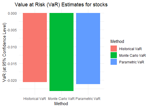
# 4.2 VaR Estimates
vaR_data <- data.frame(
  Method = c("Historical VaR", "Parametric VaR", "Monte Carlo VaR"),
  VaR = c(historical_VaR, parametric_VaR, quantile(monte_carlo_VaR, 0.05))
)

ggplot(vaR_data, aes(x = Method, y = VaR, fill = Method)) +
  geom_bar(stat = "identity") +
  labs(title = "Value at Risk (VaR) Estimates for stocks",
       y = "VaR (at 95% Confidence Level)") +
  theme_minimal() +
  theme(plot.title = element_text(hjust = 0.5))

# 4.3 Backtesting Results
# Backtesting done on 100 trading days backtesting should not exceed 5
backtest_data <- data.frame(
  Method = c("Historical VaR", "Parametric VaR"),
  Exceptions = c(exceptions_historical, exceptions_parametric)
)

ggplot(backtest_data, aes(x = Method, y = Exceptions, fill = Method)) +
  geom_bar(stat = "identity") +
  labs(title = "Backtesting Results for stock VaR Models",
       y = "Number of Exceptions") +
  theme_minimal() +
  theme(plot.title = element_text(hjust = 0.5))

# Print results
print("Historical VaR at 95% confidence level:", percent(historical_VaR_value, accuracy = 0.001), "\n")
print("Parametric VaR at 95% confidence level:", percent(parametric_VaR_value, accuracy = 0.001), "\n")
print("Monte Carlo VaR at 95% confidence level:", percent(quantile(monte_carlo_VaR, 0.05), accuracy = 0.001), "\n")
print("Number of exceptions (Historical VaR):", exceptions_historical, "\n")
print("Number of exceptions (Parametric VaR):", exceptions_parametric, "\n")

Resume & Portfolio